What Is Connective Logic?

Connective logic is a high level object oriented programming paradigm that provides an intuitive event based approach to concurrency. It underpins the Concurrent Description Language (CDL) which utilizes a dozen or so object primitives. Most engineers that have used CLiP have found that learning it is actually easier than having to become familiar with threads, locks, semaphores and sockets. In the latter case, there are a lot of other lessons that also have to be learned in order to avoid the more common pitfalls of threading and messaging. These include dealing with tortuous problems like races, deadlocks and log-jams which are amongst the most difficult bugs to repeat and locate.

(Click to enlarge...)

In practice, most programs only require minimal use of CDL in order to achieve large scalable concurrency and most existing code remains identical. This would also be true of conventional threading, but the benefit of CDL is that it operates at a much more intuitive level, and for those that find visualization useful, it can also be presented as diagrams that can then be translated into conventional source code (this significantly reduces the time taken to code parallel applications).

CDL should not be confused with UML; the latter is a completely general purpose modeling/visualization aid that addresses all areas of program (and other system) design; CLiP is a programming language (100% compile-able) with far less symbolism, and only addresses the parallel execution of concurrent software applications.

So in a sense CLiP is analogous with the form designers that GUI developers use; it only does a specific part of the job, but it does it in a way that reduces and simplifies the task. It does not require learning a complex new language, and because it localizes all concurrency issues to a few diagrams rather than being dispersed throughout the whole application, in practice only a few engineers need to become involved with it.

In order to optimize what can be done with multi-core technology, it is important to make sure that as execution progresses, any function anywhere in the system that is ready for execution, is scheduled for execution. This turns out to be a non-trivial problem for data-parallel functions with data dependent execution time and even more difficult for the general (and extremely common) case of irregular concurrency. Along with Amdahl’s law, these phenomena contribute to Intel’s rough estimate that suggests that quad core CPUs for example, are doing well if they can execute your parallelized application 3.4 times faster than its sequential equivalent (see Optimizing Software for Multicore Processors).

There are at least four considerations facing any engineer that is developing parallel code, regardless of methodology; these are granularity, exclusion, dependency and data-lifecycle. Granularity determines the size of concurrently executable functions and impacts scalability and complexity, exclusion provides techniques that prevent two or more threads of execution corrupting shared data, dependency ensures that functions cannot execute until their inputs are ready (and there is space available for their outputs), and data-lifecycles need consideration because automatic stack data cannot usually be shared between adjacent threads. This article will show how CDL deals with each of these and other issues.

Irregular dependency

In order to introduce CDL it is probably best to start with the half a dozen or so most commonly used CDL objects, and show how these can be used to parallelize most existing applications. We can start by considering the parallelization of a very simple sequential function.

If we assume for this example that all of the subroutine calls made by ‘f0’ are of sufficient ‘weight’ to justify farming out as separate tasks (granularity), and if we also assume that there are no secret data sharing issues (requiring exclusion), then the remaining considerations are dependency and data life-cycles.


   T8 f0( T1 t1, T2 t2 ) {

      T3 t3;
      T4 t4;
      T5 t5;
      T6 t6;
      T7 t7;
      T8 t8;

      t3 = f1( t1 );
      t4 = f2( t2 );
      t5 = f3( t2 );
      t6 = f4( t3, t4, t5 );
      t7 = f5( t3, t4 );
      t8 = f6( t6, t7 );

      return t8;
   }

(Click to enlarge...)

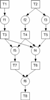
We start with a very simple function ‘f0’ which does not contain any looping or branching but we will assume that we have no way of knowing how long any of its subroutine calls are going to take because their execution times may vary according to their input data (the general case). The diagram on the right shows the dependencies for each call that the function on the left makes. The rule is simply that each subroutine call can only happen when all of its input arguments have been calculated.

If we assume that when the f0 function is executed, the two input arguments t1 and t2 are populated, this would mean that functions f1, f2 and f3 would be immediately executable (giving an initial concurrency of 3). When f1 and f2 have both executed (populating data objects t3 and t4), f5 can execute, and when f3 completes f4 can also execute. The first thing to note is that even in this simple case, without knowing execution times we cannot predict the actual runtime concurrency which will depend on whether f5 completes before f3 and so on.

In fact the diagram on the right is really just another way of expressing the sequential description on the left but in this case it makes the execution dependencies explicit, telling a scheduler what can and cannot be executed in parallel. What CDL does is to formalize this information into diagrams that can be translated into code that then ensures that at runtime f0’s subroutines will execute correctly and with as much concurrency as the calculation allows.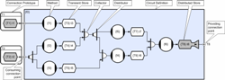

(Click to enlarge...)

This diagram is referred to as a ‘circuit’ because of its resemblance to an electronic circuit diagram, and in fact we will see that in this particular case, most of the symbolism simply reflects the information in the dependency diagram above. This example uses the following six symbols;

The method symbol represents a fragment of conventional sequential code (typically C++) and this will execute when two things have happened; firstly its inputs need to be ready, and secondly, there needs to be space for it outputs (usually the case). So in this simple example each of the methods actually represents one of the six function calls executed by the top level function f0 (these are f1 to f6). The function type is enclosed in curly braces and this is followed by its optional instance name.

The transient store symbol identifies an automatic data object which is analogous to a conventional stack object. Store buffers become writeable as soon that they are no longer referenced for read and in fact buffer depth is an attribute of the store thus enabling ‘multiple’ buffering so that writers can run ahead to the next iteration whilst readers are still using the previous iteration (this allows the construction of simultaneously active processing pipelines). The creation and destruction of buffers is transparent in CLiP and happens automatically when data is no longer referenced, but unlike Java’s garbage collection this happens continuously and deterministically (allowing real-time application development).

The collector symbol identifies a CDL object that accumulates all of its inputs and then delivers them as a single compound event. This is how CLiP applications can ensure that functions will not execute until all of their inputs and outputs are ready. In general, collection order doesn’t matter but as we shall see later when we consider persistent data stores there are cases where collection order does matter (in order to avoid deadly embraces), and where this is the case, collection order can be forced to proceed sequentially. Collection is nest-able in the sense that collections can themselves be collected and the operation is also reversible through the use of a splitter object (which breaks a compound event back into its constituent parts).

The distributor symbol identifies a CDL object that passes a reference to its input to each of its consumers (similar to publish subscribe). So in our example for instance, a reference to the t2 input is passed to the f2 and f3 functions simultaneously. When f2 and f3 have both returned from execution (and we don’t care about order) then the distributor will automatically close, which will then close its input (in this case the t2 store), and that will then enable anything blocked trying to write to t2 to execute (the expired data can be safely over-written). This style of execution is referred to as ‘event’ based (as opposed to conventional function ‘calling’) but the final result is exactly the same, it’s just that this mechanism can happen in parallel. The important point here is that all of the event management happens in the scheduler and is completely transparent to the programmer who simply needs to be able to draw a picture of what they want the scheduler to do.

Perhaps the most important CDL object is the ‘circuit’ and this is just the box that all of the other objects are contained in. The diagram above is referred to as a circuit definition, which is analogous to a class definition (and is actually translated to a class definition). As with C++ and other object oriented text languages, CLiP applications can instantiate as many instances of a definition as required. In fact as we shall see later we can also create multi-dimensional arrays of circuits and this turns out to be a very simple way of creating data-parallel applications. We can also inherit from circuits and in fact perform a number of other operations supported by OO text languages. It is the concept of compose-able circuits (and sub-circuits) that mean concurrently executing objects can in fact be just as re-usable as their sequential equivalents.

The only remaining symbol to explain is the connection prototype. This is exactly analogous to a conventional function prototype and provides a means of ensuring that circuitry is connected together correctly (data types must match). In our example, the prototype stipulates that whatever is connected to the f0 circuit, must itself be connected to stores with the appropriate data type (identified by the data type name in the curly braces). In this instance it doesn’t impose any restrictions on intermediate objects so the input may or may not have a distributor for example, and both cases would be legal.

Note that the inwardly pointing arrow on the connection points implies that the connection point is an event consumer whilst the outwardly pointing arrow implies that the connection point is an event provider. This should not be confused with read/write access.

We can now see what the f0 circuit is going to do when its inputs are provided;

f1 will execute as soon as its input is ready (a new value in t1), and there is space in t3 for its output.
f2 and f3 will both begin execution as soon as their shared input is ready (new value in t2), and space exists for their outputs (t4 and t5 respectively).
We cannot say whether all three will actually execute simultaneously because it depends on the arrival order of their input and of course the availability of space for their outputs. But the really important point is that we don’t actually care because the collectors and distributors will ensue that they will execute as soon as they can, but will never execute until they are ready. As we shall see in our next example, it is the management of this indeterminism that is the key to creating massive concurrencies without the need to become buried in complexity (see Professor Lee’s paper The Problem with Threads).
Once f1 and f2 have executed f5 becomes executable and once f3 completes f4 is similarly ready.
Finally, once f4 and f5 complete then f6 can execute and so the function completes by producing a result in f6 which will typically trigger execution of another sub-circuit which will also probably have multiple concurrency. In fact in the most general case, completion of f0 will trigger execution of more than one sub-circuit, each of which may contain their own sub-circuits, and so on. It is this compose-ability that enables CLiP applications to very rapidly accumulate very large concurrencies even in the non-trivial irregular case.
It is also worth pointing out here that most sub-circuits can actually be re-entered and if the data stores are multiply buffered, the f0 sub-circuit can actually achieve a concurrency of six under optimal conditions. If the methods f1 to f6 are stateless (do not have any instance specific data) then they can themselves be re-entered and in this case the only limit to concurrency is the number of available CPUs. Reentrancy will be dealt with in more detail in a later section.

There are a couple more points to make before moving to the next example. Firstly, as mentioned above, CDL objects are arbitrarily compose-able. Collectors can feed into distributors that than can then be fed into collectors or distributors (as well as another half dozen or so event operators) and in this way any sequential case can have an optimally parallel equivalent. Because CDL operators are compose-able, CDL circuits are compose-able and this considerably reduces the chance that applications will be afflicted by deadlocks or races and perhaps most usefully of all, because CDL primitives have known properties, and object connectivity is explicit, almost all potential deadlocks and/or races can be discovered by analysis of application circuitry (an automatable process).

As we can now see from the dependency diagram and the CDL equivalent, developing concurrent execution from sequential code can be a pretty methodical process and in most cases only requires knowledge of a few objects and some fairly simple rules. Most code remains unchanged and at no stage does the application programmer need to assume the core-count.

Example 2 – Scheduling Latency

This example is similar to the first but for purposes of illustration considers how a problem might be addressed by the proposed extensions to C++ (asynchronous function calls). In this case we consider the parallelization of a class (rather than a function) and in order to simplify the description we will use pseudo C++ syntax and imagine the existence of three functions that would make the task a bit easier. We will also assume the existence of a transparent worker thread pool that executes the asynchronously launched function calls. As in the first example, we will also assume that member functions do not share state (we’ll address this later). Consider the following very simple class which has one public member function and seven private member functions.


   class FCalc
   {
   public:
      int F( A a, B b ){
         // Transient workspace objects
         C c; D d; E e; F f; G g; H h; 
         CalcC( a, c );       // Calculate c from a
         CalcD( a, d );       // Calculate d from a
         CalcE( a, e );       // Calculate e from a
         CalcF( c, d, f );    // Calculate f from c and d
         CalcG( c, e, g );    // Calculate g from c and e
         CalcH( d, e, h );    // Calculate h from d and e
         CalcB( f, g, h, b ); // Calculate b from f, g, and h
      }
   }

Again, what we are primarily interested in here are the issues arising from dependency considerations (making sure that functions aren’t invoked until their inputs are ready), but we will also use this example to highlight some of the reasons that irregular concurrency is considered to be such a difficult problem, and in particular, why many multi-core applications fail to scale as predicted. In the two code examples that follow we have introduced 3 functions (purely for read-ability);

start( f0(a,..), f1(a,..), … );

This function is assumed to asynchronously launch each function in its argument list and automatically pass each of their respective arguments.

waitForAny( a, b, … );

This function is assumed to block until at least one of the data objects in its list is updated by an asynchronously executing function, and then return an identifier indicating (the first) value to be updated. This is therefore analogous to the Windows waitForMultipleObjects function call.

waitForAll( a, b, … );

This function is similar to the previous one but in this case it is assumed to block until all of the values have been updated.

First consider a very simple solution;

   int F( A &a, B &b ){

   // Transient workspace objects
   C c; D d; E e; F f; G g; H h;

   // Launch calcC, calcD and calcE which use ‘a’ to calculate
   // ‘c’, ‘d’ and ‘e’ repectively
   start( CalcC( a, c ), CalcD( a, d), CalcE( a, e ) );

   // Now block and wait for ‘c’, ‘d’ and ‘e’ to be calculated
   waitForAll( c, d, e );

   // Now launch calcF, calcG and calcH which use ‘c’, ‘d’ and ‘e’
   // to calculate ‘f’, ‘g’ and ‘h’
   start( CalcF( c, d, f ), CalcG( c, e, g ), CalcH( d, e, h ) );

   // Now block and wait for ‘f’, ‘g’ and ‘h’ to be calculated
   waitForAll( f, g, h );

   return CalcB( f, g, h, b );
   }

This solution is simple to create and understand but suffers from a limitation which for the purposes of this note is described as ‘scheduling latency’, and refers to the fact that because runnable tasks whose inputs are actually ready, cannot be executed immediately (the launching thread is blocked on the third result). This solution is unlikely to scale well under anything but perfect conditions. The problem stems from the fact that the first ‘waitForAll’ call is waiting for 3 results when in practice, only two are required for the calculation to progress (the application is therefore unnecessarily blocked).

This is not the same thing as Amdahl’s law which stems from fundamental limitations at the algorithmic level, but is important to raise because although it looks a lot like Amdahl’s effect, in most cases can actually be addressed.

In order to illustrate an optimal solution we need to use the waitForAny call and then use the result of each call to decide what to do next. So if for example calcC and calcD complete first we could launch calcF but if calcC and calcE finish first we could launch calcG. It might sound easy, but the following code shows just how many combinations need to be considered for the general case where all execution times are data dependent. In fact, this solution still blocks the launching thread gratuitously but this final optimization is going to be ignored here.


   int F( A a, B b ){

      // Transient workspace objects
      C c; D d; E e; F f; G g; H h;

      start( CalcC( a, c),
         CalcD( a, d), CalcE( a, e ) );
      objId = waitForAny( c, d, e );

      if ( objId == c ){
         objId = waitForAny( d, e );
         if ( objId == d ){
            start( CalcF( c, d, f ) );
            objId = waitForAny( e );
            start( CalcG( c, e, g ) );
        }
         else{
            start( CalcG( c, e, g ) );
            objId = waitForAny( d );
            start( CalcF( c, d, f ) );
         }
         start( CalcH( d, e, f ) );
      }
      else if ( objId == d ){
         objId = waitForAny( c, e );
         if ( objId == c ){
            start( CalcF( c, d, f ) );
            objId = waitForAny( e );
            start( CalcH( d, e, h ) );
         }
         else{
            start( CalcH( d, e, h ) );
            objId = waitForAny( c );
            start( CalcF( c, d, f ) );
         }
         start( CalcG( c, e, g ) );
      }
      else{
         objId = waitForAny( c, d );
         if ( objId == c ){
            start( CalcG( c, e, g ) );
            objId = waitForAny( d );
            start( CalcH( d, e, h ) );
         }
         else{
            start( CalcH( d, e, h ) );
            objId = waitForAny( c );
            start( CalcG( c, e, g ) );
         }
         start( CalcF( c, d, f ) );
      }

      waitForAll( f, g, h );

      return CalcB( f, g, h, b );
   }

The circuit below illustrates a CDL solution and introduces a few more properties of the technique;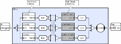

(Click to enlarge...)

In the first example, the subroutine calls (f1 through f6) used CLiP methods which means that although these can execute in parallel with each other, each actual method invocation executes sequentially (so the potential concurrency is six). In many cases, the translation to CDL can continue to finer granularity and in the above diagram we have assumed that this is the case. This would obviously increase concurrency but would also increase scheduling overhead and deciding how far down to take CDL is an important design decision.

Although the sub-circuits in this example all happen to have one input and one output, this is not a restriction imposed by CDL, and they can in fact have an arbitrary number of entry points (equivalent to public member functions), and each of these can have any number of inputs and/or outputs.

The CalcC, CalcD and CalcE sub-circuits are white and the CalcF, CalcG and CalcH sub-circuits are colored gray. This is because in this example, the first 3 are members of the parent circuit and exist as instances with their own state, whilst the gray sub-circuits are actually ‘calls’ to remote circuits that are instantiated somewhere else in the application. In the latter case these are typically references to sub-circuits on remote machines and the technique is provided for cases where circuits need access to particular devices (disks, sensors etc), or equally often because of specialist processing issues like those arising when high performance applications need to offload to specialist processing devices like an IBM Cell BE, ClearSpeed card or GPU. This would be analogous with a Service Oriented Architecture (SOA) view of the world.

Before moving on the next example, it is worth considering how the complexity of the two approaches can scale. In the optimal asynchronous solution above, 30 to 40 lines of code were required for an irregular problem with a concurrency of three. If the concurrency is increased to four, about 4 x 30 lines are needed, if concurrency is increased to 5 then about 5 x 4 x 30 (600 lines) are required and complexity continues to grow with factorial scaling.

The circuit below addresses the case with concurrency four, but in this case, complexity scales linearly (in terms of the required number of objects and connections). In this particular example however, the number of crossed lines means that the diagram can become confusing and this example therefore introduces the notion of a conduit connection. In this case all connections to the conduit sharing common labels (in this case C, D, E, or F) are made. So in this case for example, GSUB’s collector will collect inputs from the d, e, and f transient stores and when all three are ready, GSUB will be triggered.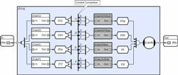

(Click to enlarge...)

This illustrates a useful property of connective logic which is that timing indeterminism is addressed by the scheduler and not by the engineer. This simplifies the parallelization of the general irregular concurrency case considerably, and when this is combined with its other significant property (circuitry is compose-able) the task of achieving highly scalable applications under typical conditions becomes attainable for most applications.

Example 3 – Exclusive Data Access though Scheduling

Broadly speaking there are two ways of addressing the problem of data races (where two threads of execution are able to access the same data inconsistently) and these are; scheduling exclusion, and data arbitration. In the first case, it is necessary to ensure that two pieces of code that access the same data are never scheduled simultaneously, and in the second, some kind of arbitration scheme that is associated with particular groups of data is required. In the arbitration case, a blocking scheme (usually called a lock or mutex) could be used, or alternatively one of the more recent techniques based on the concept of STM (software transactional memory) could be used. CDL supports both approaches but at the time of writing has yet to adopt STM for the latter.

In order to address this topic it is necessary to introduce two new CDL objects referred to as a multiplexor and a de-multiplexor. Like all CDL objects they have a concept of re-entrancy which determines the number of times that they can be simultaneously opened by provider/consumer pairs. Re-entrancy is an advanced topic that will not be discussed here, but in the special case where the de-multiplexor has a concurrency of one, they can be used as means of serializing pieces of code that we do not want to execute in parallel.

We can illustrate this by making a small modification to the previous example and thereby ensure that CalcC, CalcD and CalcE will never execute in parallel (although they can still execute serially in any order).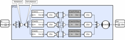

(Click to enlarge...)

The explanation is as follows. When a new value is delivered to the circuit, it is replicated three times by the distributor and then serialized as three events by the multiplexor. The de-multiplexor then passes each event to the appropriate sub-circuit which then executes sequentially with respect to the two adjacent sub-circuits (but in parallel with all non-excluded circuitry). Note the use of labels on the links (C, D and E) which are used to map multiplexor inputs to de-multiplexor outputs.

Although not relevant to this example, if we raised the de-multiplexor concurrency to two (a creation attribute) then the sub-circuits would be able to execute two at a time, and if we raised it to three, we would be back to full parallel execution (therefore a bit pointless!).

Example 4 – Exclusive Data Access though Arbitration

The previous example provides a safe compose-able technique for avoiding data-races but unless the application’s concurrency exceeds the core count of the target hardware, it could reduce overall performance by introducing a convoy effect. Under these circumstances a finer grained exclusion scheme is required and this introduces another CDL object referred to as an arbitrated store (AST).

To continue the class/circuit analogy, ASTs are used as repositories for circuit state (analogous to object state). There is no limit to the size of data object that they arbitrate and again the decomposition of state into smaller grain ASTs is another important design consideration. Coarse grain store schemes are easier to manage, but finer grain schemes are less like to introduce unnecessary scheduling latencies through convoy effects.

ASTs differ from their transient equivalent used in earlier examples in that their data persists (isn’t invalidated when no longer referenced) and access to their data is restricted by one of a number of configurable exclusion schemes. Typically, stores allow any number of readers, or one writer, but if the store is double buffered then readers can access the current value whilst one writer is updating the other which then becomes the current value for subsequent read accesses. This provides safe arbitration and greatly reduces blocking; which can only occur if more than one simultaneous write/update is attempted.

However, because multiple writers could still block, this could lead to deadly embraces in exactly the same way that conventional locks do (the store has no implicit advantage over other problematic schemes). But in practice they seldom occur because most AST access sequences are achieved through the use of CDL’s ordered collectors (which ensure that stores are only accessed using particular sequences). Because all CDL objects have a notion of scope, data stores can be made inaccessible through anything other than published schemes.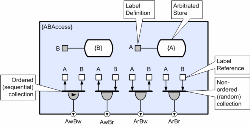

(Click to enlarge...)

This example illustrates how such schemes can be created and implemented. Note that in the example above, it is assumed that the store has been configured so that reads will never block, and writes/updates will only block if more than one simultaneous write/update is attempted (requires multiple buffers).

This example introduces the arbitrated store object and also the concept of labels and references. The shaded boxes define named labels, and the un-shaded (white) boxes represent references to them. So in this case, each collector is actually connected to both stores.

Also note, that because of the particular arbitration scheme used by this example circuit, only when A and B are simultaneously opened for write, could a deadlock occur and that is why only the AwBw collector needs to be ordered. Provided the stores are only accessed through these four entry points, deadlock cannot occur. The same approach applies in the general case where collections of collections of stores are required (collectors are nestable).

In the case where stores are publicly exposed (and sometimes there are good reasons for wanting to do this), then the CDL translator will spot most deadly embraces through analysis of connectivity. The only cases that the analyzer cannot detect are cases where methods access arbitrated stores for write during their execution and whilst this is permitted it is seldom required.

Another issue that often arises with persistent data is consistency. It could be that we have a long processing chain, and in order for program logic to work, all stages must use a consistent latest value. Although we want readers to see a consistent value, we don’t want to block updaters, and we may need the value to stay consistent for relatively long periods.

Under these circumstances it is quite common to use a distributor to ensure that each stage of the calculation uses the same AST date instance, and in practice this does not prevent the store being written to (e.g. from the GUI thread), and indeed it can do so any number of times without the need for data to be locked throughout a complete iteration. This avoids the convoy effect that can occur if a data object needs to be protected from change for extended periods (coarse locking). It also saves bus bandwidth by avoiding the need to make multiple gratuitous copies of the data object between stages in the processing chain.

When the last stage of the chain (F3) completes, the distributor will close, and this will then allow any writes/updates that occurred during the processing of the chain to become the ‘current’ value.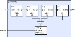

(Click to enlarge...)

One final point is that collectors do not behave in the same way that a sub-routine requesting a series of locks would behave because incomplete collections requested by CLiP methods do not block the execution of any particular worker thread whereas conventional threading models will block if any of the locks in the sequence are unavailable (although this may well turn out to be avoidable by a successful conclusion to current research with STM).

In fact CLiP method scheduling uses a technique that means that worker threads only ever block if the number of executable tasks dips below the number of available CPUs, or if the method explicitly accesses block-able objects (unnecessary but sometimes useful). This reduces context switching overhead as well as stack usage and is described in the ‘holographic processing’ paper that accompanies this.

Example 5 – Data Parallel Execution

This last example addresses the more familiar territory of data-parallel applications. This case is considered to be more ‘familiar’ than those dealt with earlier because historically, high performance computing has tended to involve this type of technique (although this will arguably change with the arrival of multi-core). This section looks at how CLiP deals with the data-parallel sections of general concurrent applications.

Before moving to an actual example it is probably useful to differentiate various levels of data-parallelism. Firstly there is the most specialized case of all; Single Instruction Multiple Data (SIMD) which will execute efficiently on GPUs and other accelerator devices. Common applications are pixel rendering, Fast Fourier Transforms (FFTs) and numerical filters.

If a function branches on data (includes statements like ‘if’, ‘switch’, ‘while’, or data dependent length ‘for-loops’) then it is more likely to be a Multiple Instruction Multiple Data (MIMD) or some other more general class of problem and what this means is that it is going to be a lot more difficult to scale efficiently.

Since this latter case is considerably more typical of day to day programming requirements, the chosen example falls into this more general category and highlights some of the reasons that multi-core applications are not expected to scale linearly even in this idealized case. The example highlights how a form of scheduling latency can often be a major cause and explains a CDL technique for avoiding it. However, it is important to point out that this is not the only obstacle to perfect linear scalability and there are others relating to sheer physical constraints like bus bandwidth which CLiP will have no special means of avoiding.

This example is specifically picked to highlight something that it can address which is a problem that arises from the use of processing barriers such as those employed by scatter/gather type mechanisms and others provided by OpenMP and MPI type approaches. As with the asynchronous programming approach discussed earlier we are not necessarily saying that scheduling latency cannot be minimized using these technologies, but we are pointing out that to achieve it may require an unexpected amount of effort.


void MatToColRow::Calc( A Input[N][M], B Rows[N], C Cols[M] ){
   D Grid[N][M];
   for ( i = 0; i < N; i ++ ){
      for ( j = 0; j < M; j ++ ){
         CalcGrid( Input, i, j, Grid );
      }
   }
   for ( i = 0; i < N; i ++ ) {
      CalcRow( Grid, i, Rows );
   }
   for ( j = 0; j < M; j ++ ) {
      CalcCol( Grid, j, Cols );
   }
}

The example above is probably fairly typical of the sort of code that will need to be migrated to multi-core over the coming years. But even if we assume that it is embarrassingly parallel (no dependency between iterations) there are a number of issues that could prevent it from scaling in the general MIMD case where the execution time of each function call is dependent on its data. And it is generally true to say that the more exaggerated the variability, the less well it will perform.

Firstly there is the obvious point that if the loop count isn’t divisible by the number of cores then different CPUs will end up performing different numbers of tasks, and secondly, if each task takes a different number of cycles then we have no way of knowing how each loop will run down as it synchronizes each of its CPUs. The point is that as each thread synchronizes at the end of the loop, parallelism will drop from ‘N’ (typically the number of cores) all the way down to one (there has to be a last thread to complete) and while this is happening the scaling has to be less than N to 1 (not all CPUs are executing). So how can we avoid processing barriers and keep the concurrency above the core count?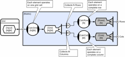

(Click to enlarge...)

The circuit above has the same functionality as the three loop example above that, but in order to explain how it works it is necessary to briefly introduce CDL’s tensor style notation (connections between multi-dimensional objects). Without going into too much detail, the default rule is that repeated dimensions connect one to one (those shared by provider and consumer), whilst residual dimensions imply many-to-one operations like collection, multiplexing, distribution etc (the precise operation depends on the particular provider/consumer pair). It is worth mentioning that defaults can be over-ridden and irregular cases are supported, but this is only seldom required in practice for typical data-parallel applications.

(Click to enlarge...)

In the example circuit above, each element of the [N] dimensioned collector therefore collects [M] elements from the grid (corresponding to a complete row). Conversely, each element of the [M] dimensioned collector therefore collects [N] elements from the grid (corresponding to a complete column).

So the example circuit has the property that as the two dimensional grid becomes populated by the calcGrid method, each row calculation eventually collects a complete row’s worth of input, and each column calculation eventually collects a complete column’s worth of data. There is no concept of a processing barrier and so the row and column calculations can proceed in whatever order their non-deterministic completion order dictates. This is important because in the worst case a scheme that chooses to calculate the complete grid first, then all rows, then all columns; could in the very worst case have all columns except one available to execute (i.e. all inputs ready) but be completely stalled because it chose to execute rows first (and there are none actually ready). The worst case is unlikely to occur often, but then so is the best case, the CDL solution exhibits optimal scheduling latency in all cases.

With the CDL solution, row and column calculations become executable even before the complete two dimensional grid has been populated, and their completion order does not limit progress. Concurrency is further liberated by the likelihood that in this particular example, the grid calculation can also be re-entered whilst the row and column calculation (and even residual grid calculation) are still proceeding for the previous iteration.

This concludes the overview of the connective logic programming paradigm, and interested readers are invited to read the accompanying paper that explains how CDL is executed by its associated runtime (holographic processing).